Fun With Science / Globe Deconstruction / Section · pages 415–473
What the Compass Measures in Antarctica
Antarctica’s Magnetic North, pp. 415–473 — the suggestion that magnetic declination is an invention, and the ring magnet a flat plane would need in its place.
A compass at Scott Base points 140° away from the noon Sun. No map is involved in that.
His four declinations: right to a tenth of a degreeDeclination as an invention: the record is older than the mapsA ring magnet: excluded by his own tableThe map itself: his labelled speculation, not graded
Where this lands
The four numbers he reads off the NCEI calculator are correct, and they are measurements, not conventions. Declination is the angle between where a compass needle points and where the sky turns about — the noon Sun on either model, or Polaris, which the flat model itself puts over the centre of the plane. At his site A on Ross Island that angle is 135°; at Scott Base, 95 km away, it is 140°, because this close to the dip pole the needle swings by degrees over tens of kilometres. It was logged by navigators a century before Newton and found to change in 1634; it cannot have been invented to protect maps that did not yet exist. A compass that “works properly across the entire Earth” in the chapter’s sense — pointing at one place — is what a magnet under the centre of a flat plane gives, everywhere: zero declination at all four of his sites, not 135° east of true north at one and 130° west at another 1,326 km away. The same magnet fails the dip needle, the intensity map and the fall-off with height, and no depth mends all three. The map that removes declination is his own rough draft, stamped speculation, and this page leaves it there.
What the claim is
p. 452, under the heading Magnetic error = reality?: “What happens when we assume that the compass does indeed work properly across the entire Earth? What if magnetic declination was a concept created to make our current maps appear accurate? Was it used to remove our trust in the compass? What if the compass was right all along? Antarctica confirmed my suspicions.” The confirmation, at p. 454, is a table of four Antarctic sites with their declinations read from the NCEI geomagnetic calculator: A at 77°03′S 168°09′E, 135°07′E; B at 78°08′S 110°31′E, 130°30′W; C at 70°18′S 24°27′E, 40°10′W; D at 72°10′S 74°01′W, 26°18′E. Each site is then drawn with its magnetic north rotated onto geographic north, the coast is turned to match, and the result is the “Magnetic Declination Removed” flat map at pp. 463–464, which the book labels “speculation, still a work in progress” and offers as a rough draft.
The map’s purpose is stated in the book’s own words, in the caption at p. 463: “The end goal is to create a map that does not rely on star visual gemometry.” That is the crux, because declination is by definition the needle’s angle from the sky: a map that removes it is a map that has decided, in advance, not to be checked against the stars. And the inspiration named in the chapter’s first sentence, Urbano Monte’s ten-foot planisphere of 1587, is drawn on a north-polar azimuthal projection — a globe flattened about its pole, which Monte designed to be mounted on a board and turned about a pivot at the centre, and which he describes on the sheets as a way of showing the sphere on a flat surface.
Two things are being claimed, and they come apart. The first is about a measurement: that declination is not a property of the world but a correction invented to save the charts. The second is a map built on the first. The map is fenced by its author and this review does not grade it. The measurement claim is testable, and the test does not need a map.
What declination is, and what it is not
A compass needle settles along the horizontal part of the local magnetic field. True north is something else: the direction on the ground toward the point the sky turns about, which is also the direction of the Sun at local noon, when it is highest. Both models agree on that second definition. On a globe the noon Sun lies along the meridian toward the pole; on the flat plane of the book, the Sun circles above the disc and is nearest — highest — when it stands on the observer’s own radius, so the noon direction is toward the centre. Either way, stand at Scott Base at local noon, point one arm at the Sun and lay a compass on the other, and the two point 140° apart. That angle is declination. It exists before anyone draws a map, and it would exist if every map were burned.
North of the equator there is an even simpler reference, and it is the book’s own. The flat model puts Polaris above the centre of the plane; on a globe it stands within a degree of the celestial pole. On either account, a compass that “works properly” in the chapter’s sense points at Polaris. Stand outside on any clear night with a compass: in Boston the needle sits 14° to the left of the star, in Chicago 4°, in Denver 7° to the right, in Seattle 15°; in Erie, where the book’s eclipse footage was taken, 9° to the left. That is declination, read off the sky in a minute, and it was being read that way in Song-dynasty China, where Shen Kuo recorded in 1088 that the needle “always inclines slightly to the east” of true south, four centuries before Columbus watched his own needles drift from the star as he crossed the Atlantic.
The chapter’s test therefore has an answer that does not touch cartography. If the compass “was right all along” — if it points at true north — then declination is zero everywhere and the four numbers on his own table are wrong. If the four numbers are right, the compass does not point at true north in Antarctica, and no rearrangement of the coastline changes where the noon Sun is.
His four numbers, reproduced
The NCEI calculator he used runs the World Magnetic Model. The open sibling of that model is the International Geomagnetic Reference Field, now in its fourteenth generation, fitted to the same data: about a hundred and fifty ground observatories, repeat-station surveys, and the three Swarm satellites. Running IGRF-14 for September 2026 at his four sites gives:
| site | position | his declination (NCEI) | IGRF-14 | dip | intensity |
|---|---|---|---|---|---|
| A | 77°03′S 168°09′E — Ross Island | 135°07′E | 135.0°E | 80.4° up | 62.2 µT |
| B | 78°08′S 110°31′E — East Antarctic plateau | 130°30′W | 130.6°W | 77.2° up | 59.8 µT |
| C | 70°18′S 24°27′E — Dronning Maud Land coast | 40°10′W | 40.2°W | 61.7° up | 40.4 µT |
| D | 72°10′S 74°01′W — Alexander Island | 26°18′E | 26.3°E | 62.8° up | 44.3 µT |
The declinations agree to a tenth of a degree. So do the two columns he did not print, and they matter more than the one he did. At A the needle is not only 135° off true north; it is trying to point almost straight up, 80° out of the horizontal, and the horizontal part it can follow is a sixth of the total. At C, on the far side of the continent, the tilt is 62° and the field is a third weaker. Sites A and B are 1,326 km apart on a continuous ice sheet — the McMurdo–South Pole traverse crosses that ground every season — and their needles point 94° apart in true bearing. Whatever produces that is not pointing at one place.
How the field is measured
The calculator is the last step of a chain, and the chain is worth setting out because the chapter treats its output as a single institutional pronouncement. It is closer to the opposite: the most continuously and independently measured quantity in the physical sciences, by instruments that share nothing but the field.
The compass and the dip needle. Declination was noticed by Columbus in 1492, when his needles drifted from the pole star as he crossed the Atlantic. Dip — the needle’s tilt out of the horizontal — was measured in London by the instrument-maker Robert Norman in 1581 at about 72°, and in 1600 William Gilbert’s De Magnete reported that a small dip needle moved over a spherical lodestone, his terrella, tilts exactly as needles tilt across the Earth: level at the sphere’s equator, vertical at its poles. That is the founding observation of the subject, and it is a shape observation. In 1634 Henry Gellibrand compared his London declination with William Borough’s of 1580 and found it had moved from 11°E to 4°E: the field changes. Edmond Halley crossed the Atlantic twice in the Paramore, 1698–1700, to measure declination for navigators and published the first chart of lines of equal declination in 1701. All of this precedes the maps the chapter says declination was invented to protect; most of it precedes Newton.
Absolute intensity. Until 1832 a needle could only compare one field with another. Gauss showed how to measure its strength in absolute units with a bar magnet, a balance and a clock, and the Magnetic Union he ran from Göttingen with Weber put observatories on a common schedule across Europe. In 1839 he fitted the data with spherical harmonics and showed that the field’s source is inside the Earth and dominantly a single dipole — the same analysis IGRF still performs.
Observatories. About a hundred and fifty stations record the full vector continuously with fluxgate and proton-precession magnetometers and share it through INTERMAGNET: Hartland, Eskdalemuir and Lerwick in Britain; Boulder and Fredericksburg in the United States; in Antarctica, Dumont d’Urville, Mawson, Casey and Scott Base among others. Their instruments are absolute: a proton magnetometer measures a precession frequency and the field strength follows from a constant of nature, not from a calibration anyone can adjust.
Surveys on foot, by ship and by aircraft. National surveys re-occupy repeat stations every few years; ships towing magnetometers mapped the sea floor in the 1950s and 60s and found the striped record of past reversals that became the Vine–Matthews–Morley test of sea-floor spreading; aeromagnetic surveys, flown for minerals, cover most continents and, through the ADMAP compilation, most of Antarctica.
Satellites. Magsat in 1979–80, Ørsted from 1999, CHAMP from 2000 to 2010 and the three Swarm satellites since 2013 measure the vector field from orbit, at about 450 km, several times a day over every part of the Earth. They are the reason the models can be global at all.
Users with no stake in the theory. Runways are numbered by magnetic heading, and are renumbered as declination drifts: Tampa International repainted 18R/36L as 19R/1L in 2011. Every marine chart carries a compass rose with the local declination and its annual change. Every aircraft has a compass-swing record. And the phone in a reader’s pocket holds a three-axis magnetometer that reads dip and total intensity directly; laid flat, the vertical component is the dip, and either can be compared with the model for the reader’s own address in an afternoon. That last one, and the compass held up to Polaris, are the self-tests this page recommends before any other — with one caution on the phone: its magnetometer is thrown by nearby steel and needs the figure-of-eight calibration the compass app asks for, so hold it away from the desk and any metal, and take three readings rather than one.
These do not agree because they are told to. They agree because they are measuring the same thing, and what they measure is the shape of the field.
What the measurements describe
Seven quantities describe the field at a point, and the model gives them anywhere. Two of them, mapped:
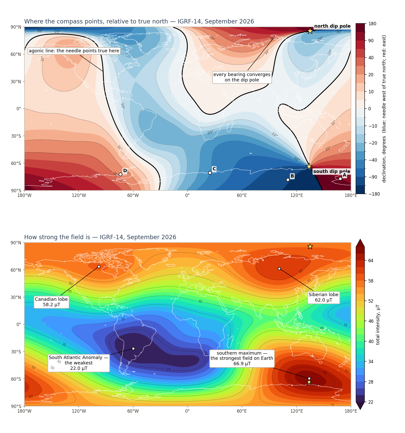
And some of what they show at the surface, in numbers, from the same IGRF-14 run:
| quantity | measured (IGRF-14, 2026) | what a single tilted dipole predicts |
|---|---|---|
| dip by latitude, longitude-mean | +88° at 90°N, +75° at 60°N, +47° at 30°N, −9° at the equator, −54° at 30°S, −68° at 60°S, −72° at the South Pole | tan I = 2 tan &lambda: vertical at the magnetic poles, level at the magnetic equator, 60° at 41° magnetic latitude |
| where the needle stands vertical | two points: 85.4°N 133.5°E and 63.8°S 134.8°E, the second in the Southern Ocean off Adélie Land | two points, antipodal to within the non-dipole part |
| strongest surface field | 66.9 µT at 59.5°S 134°E; the strongest in the north is 62.0 µT, in Siberia | equal at the two poles; the difference is the non-dipole field, and it favours the south |
| weakest surface field | 22.0 µT at 26.5°S 60°W, the South Atlantic Anomaly | half the polar value round the magnetic equator |
| fall-off with height, surface to 450 km | 0.818 over Hartland, 0.802 over Scott Base, 0.779 over the Gulf of Guinea | (a/(a+h))3 = 0.815 |
| axis | the dipole part is tilted 9.2° from the rotation axis | a dynamo in a rotating fluid core aligns with the rotation |
| change | north dip pole 2,570 km from where James Clark Ross stood on it in 1831; south dip pole 1,268 km from where David, Mawson and Mackay reached it in 1909; dipole strength down 7.6% since 1900 | a fluid dynamo drifts and decays; a permanent magnet does neither |
The pattern Gilbert saw on his terrella is the pattern in the first row. A needle that stands up at two points and lies flat on a band between them, with the field twice as strong at the ends of that axis as in the middle, is the field of a magnetised sphere, and it has been that since 1600. What the four centuries since added is the reason: the crust cannot be the magnet, because magnetite loses its magnetism above 580 °C and rock reaches that temperature about twenty to thirty kilometres down, so a permanently magnetised layer can only be a thin skin, and the anomalies that skin produces are a few hundred nanotesla, a percent of the whole. The source is deeper, where nothing can be permanently magnetised, so it must be an electric current: the convecting, conducting outer core, whose existence seismology establishes on its own from the shadow it casts in shear waves. A current system in a rotating fluid is organised by the rotation — the flow lines up in columns parallel to the spin axis — which is why the magnetic axis sits within nine degrees of the geographic one and, averaged over thousands of years in the rock record, on it. Every one of those facts is a globe fact. Not one of them was collected to argue with a flat plane.
Two more witnesses, one needing no instrument at all. The aurora australis forms an oval two to three thousand kilometres across, centred near the south geomagnetic pole: seen from Tasmania and the south of New Zealand and from the stations beneath it, and not, on the same night, from South Africa or Argentina except in a storm. A pole spread round the rim would light the whole 126,000 km of Antarctic coast at once. And on the author’s own ground: the same model, run at its 1902 epoch — the coefficients fitted to the observations of that era, Scott’s Discovery magnetic hut at Hut Point among them — puts the field at Hut Point at 68.8 µT with the needle 86° from level; today it is 62.0 µT and 80°. A tenth of the field gone in a century and a quarter, on the ice the chapter is about. A convention does not decay; a fluid dynamo does. The observed Discovery values, rather than the model’s reconstruction of them, are still to be added.
The ring magnet a flat plane needs
The flat model has to supply a field in which a compass points toward the centre of the plane from everywhere on it, since that is what “the compass was right all along” means. The arrangement the flat model’s own literature offers is a magnet with one pole under the centre — the Arctic — and the other running round the rim, under the Antarctic coast: a ring. The Flat Earth Society’s wiki answers the question How is there a magnetic field? Magnets can’t be unipolar with exactly this, a radially magnetised ring of the kind found in loudspeakers, “one magnetic pole at the center and the other at all points on the edge,” which it says “perfectly replicates what is found on the Earth.” The other shape sometimes drawn, a bar magnet standing on end under the centre, is the ring shrunk to a point beneath it: it is axisymmetric too, so it fails the direction test identically, and with its far pole buried it leaves the rim weaker still — 2% of the centre, with the needle at 70°S only 20° from level, for a 10,000 km bar whose top sits at the depth that fits the satellites. Three things are wrong with it, in increasing order of strength.
Nothing natural makes one
Permanent magnetisation in nature is grains of magnetite in rock, magnetised by the field they cooled in or, for the lodestones Gilbert used, by lightning. It is weak, it is shallow for the Curie-point reason above, and it is set by whatever field already existed, so it cannot be the origin of that field. A ring forty thousand kilometres across with a pole at its centre is not a form any process produces, and a permanent magnet of any shape does not move its pole 2,570 km in two centuries, lose 7.6% of its strength in one, or reverse, as the sea-floor stripes record the field doing hundreds of times.
Even granted, it points the wrong way
A ring with a pole at its centre is symmetric about that centre, and the horizontal part of a symmetric field is radial. A compass on that plane points at the centre from everywhere: declination zero at A, zero at B, zero at C and D. The book’s own table says 135°E, 130°W, 40°W and 26°E. A modeller can break the symmetry by adding more magnets and tuning them until the compass points 135° off at Ross Island — but then the compass no longer points at the centre, declination is real, and the premise of the map is gone by construction. The ring cannot both explain his table and remove it.
Even allowed the wrong direction, it fails on strength and tilt
Suppose the direction is waved through. The rest of the needle’s behaviour is still there to be matched, and the script below computes it for a magnet whose two poles have the equal and opposite strength every magnet’s must — flux that leaves one pole arrives at the other — with the ring pole spread round the rim, for magnet depths from 1,000 to 10,000 km:
| magnet depth | needle level at | equator ÷ north pole | rim ÷ north pole | dip at 70°S | 450 km ÷ surface, over the centre |
|---|---|---|---|---|---|
| 1,000 km | 29°S | 0.011 | 0.016 | 18° up | 0.476 |
| 2,000 km | 30°S | 0.041 | 0.031 | 30° up | 0.666 |
| 4,178 km | 33°S | 0.155 | 0.063 | 36° up | 0.813 |
| 6,371 km | 38°S | 0.290 | 0.095 | 30° up | 0.867 |
| 10,000 km | 50°S | 0.475 | 0.147 | 16° up | 0.906 |
| measured | about the equator | 0.59 | above 1 (66.9 against 62.0 µT) | 62° to 80° up at his four sites | 0.80–0.82 |
Read across any row. A point pole under the centre falls off as the inverse square of distance, so the field at the equator is a small fraction of the field at the pole unless the magnet is buried thousands of kilometres deep, and burying it that deep pushes the level-needle line into the southern mid-latitudes, where no dip needle has ever read zero. The rim pole is the same strength as the centre pole but smeared round a circumference of 126,000 km, so the field along the Antarctic coast comes out at between two and fifteen percent of the field at the centre. Measured, the southern field is the strongest on Earth: 66.9 µT south of Australia, against 62.0 at best in the north, and 62 µT at Ross Island itself. And the dip across Antarctica in the ring model is shallow — 16° to 36° at 70°S, because the needle there is caught between a weak nearby rim and a strong distant centre — where his own four sites read 62° to 80°. The one depth that reproduces the satellite fall-off, 4,178 km, gets the equator wrong by a factor of four, the rim by a factor of sixteen and the dip at his four sites by between twenty-six and forty-four degrees. No depth mends more than one column.
The southern field is the decisive column, and it is the one a reader can hold in one sentence. A ring puts its second pole round the longest circle on the map; the field there has to be the weakest on the plane. It is measured to be the strongest on the Earth.
What removing declination would do
The map at pp. 463–464 rotates each stretch of Antarctic coast until its compass reads true. Applied consistently — and the chapter’s premise is that it should be, since the compass “works properly across the entire Earth” — the same rule turns Boston 14° one way and Seattle 15° the other, a 29° twist across a continent whose roads, railways and property lines have been surveyed against the stars for two centuries and do not twist. It puts London 24° from where it was in 1810 and 11° the other side of it in 1580, since the declination there swung through 35° between Elizabeth I and George III while the city stayed where it was. And it makes the south dip pole, which a sledging party reached on the ground in January 1909 at 72°25′S 155°16′E with the needle standing vertical, a circle round the whole coast rather than a point — and then has no account of why the point has moved 1,268 km out to sea since.
The other side of it
The strongest form of the chapter’s position is not that the numbers are false but that they are his opponents’ numbers: the model behind the calculator is built by the agencies whose maps are in question. Three replies, in order of how little they concede. First, the raw quantity is not a model output. Declination at a site is a compass, the noon Sun and a protractor; dip is a needle on a horizontal pivot; intensity is a proton magnetometer, whose reading is a frequency. Anyone in Antarctica can take all three in an afternoon, and expedition parties have been doing so since 1841. Second, the historical record was made by people with the opposite incentive: a navigator who logged a wrong declination ran his ship onto rocks, and the Admiralty gave Halley a ship to chart it because navigators needed it. Third, the values he printed were the values he needed — the chapter accepts them as data for the map. A theory cannot use a measurement as its input and call the same measurement an invention.
A weaker but fair objection is that satellite data can be set aside by a reader who does not accept satellites. It can; this page does not need it. Drop the last column of the ring table and the other four still fail, and every entry in them is a surface measurement with a nineteenth-century instrument.
What the chapter does get right should be said. The compass genuinely is close to useless across most of Antarctica — the horizontal component at Ross Island is a sixth of the total and the needle is sluggish and wrong — which is why polar navigation moved to sun compasses, gyros and grid north long before GPS. Grid north is a convention — the map’s vertical lines taken as north across the whole continent — adopted precisely because the compass fails there: the one place people actually gave up on the compass is the place the chapter says the compass was right. That is a real fact about the field, and it is a fact the ring magnet cannot produce either: it needs the south dip pole to be a single point on the far side of a magnetised sphere, so that the needle over a whole continent is pulled nearly vertical by the pole’s nearness while its horizontal remnant swings through every bearing round it. His four sites, read with their dips, are that picture.
What would change our mind, and where this page could be wrong
A compass in Boston or Seattle that points at Polaris. A compass at Scott Base that points at the noon Sun. A dip-needle traverse along the Antarctic coast reading the same tilt all the way round, as a rim pole requires, rather than standing vertical at one point off Adélie Land and leaning 62° at his site C. A surface intensity survey in which the southern field is weaker than the northern. A declination record that begins only after the maps it is said to protect, rather than in 1492. A natural process that produces a ring-shaped permanent magnet, at any scale. Any of these would send this page back for rewriting.
Where it could be wrong now: the historical values quoted for London — 11°E in 1580, 4°E in 1634, 24°W around 1810 — are taken from the standard compilation of the London series and not yet from the original observations; the position of the 1909 party is Mawson’s figure and later re-analysis moved it by a few tens of kilometres; and the ring model is one shape of flat-plane magnet, chosen because it is the one the flat model’s own wiki draws, with the vertical bar as the only other shape computed. A third shape would need to be computed on its own. None of that reaches the two findings that carry the page: the four numbers are right, and a field that points at one place cannot produce them.
Reproduce it
Everything above comes from one script, antarctica_magnetic.py, which needs only numpy and the ppigrf package that carries the IGRF-14 coefficients. It prints his four sites against the model, the field at a dozen other places, the two dip poles and the intensity extremes, the fall-off to 450 km, and the ring-magnet table for five depths. Change the date, the sites or the magnet depth and the tables follow.
Sources & further reading
- Levi Miller, Globe Deconstruction? — prerelease draft, 2026: pp. 452 (the claim), 454 (the four sites), 463–466 (the MDR map and its labels).
- Alken, P. et al., “International Geomagnetic Reference Field: the thirteenth generation,” Earth, Planets and Space 73, 49 (2021); IGRF-14 coefficients, IAGA Division V-MOD, 2024, ncei.noaa.gov. The NCEI calculator the book used: Magnetic Field Calculators.
- Laundal, K. M.,
ppigrf— pure-Python IGRF, github.com/IAGA-VMOD/ppigrf. - Shen Kuo, Dream Pool Essays (Mengxi Bitan, 1088), on the magnetised needle and its easterly inclination; Needham, J., Science and Civilisation in China, vol. 4 part 1 (1962), §26(i).
- Gilbert, W., De Magnete (1600), Book V, on dip and the terrella. Norman, R., The Newe Attractive (1581). Gellibrand, H., A Discourse Mathematical on the Variation of the Magneticall Needle (1635). Halley, E., A New and Correct Chart Shewing the Variations of the Compass in the Western & Southern Oceans (1701).
- Malin, S. R. C. and Bullard, E., “The direction of the Earth’s magnetic field at London, 1570–1975,” Phil. Trans. R. Soc. A 299 (1981) — the London declination series.
- Gauss, C. F., Intensitas vis magneticae terrestris ad mensuram absolutam revocata (1832); Allgemeine Theorie des Erdmagnetismus (1839).
- Ross, J. C., “On the position of the North Magnetic Pole,” Phil. Trans. R. Soc. (1834). Shackleton, E., The Heart of the Antarctic (1909), vol. 2, David’s narrative of the northern party’s arrival at the south magnetic pole, 16 January 1909.
- INTERMAGNET, intermagnet.org; British Geological Survey observatories at Hartland, Eskdalemuir and Lerwick; ESA Swarm mission, earth.esa.int.
- Vine, F. J. and Matthews, D. H., “Magnetic anomalies over oceanic ridges,” Nature 199 (1963).
- Golynsky, A. V. et al., “New magnetic anomaly map of the Antarctic” (ADMAP-2), Geophys. Res. Lett. 45 (2018).
- Federal Aviation Administration, Tampa International Airport runway redesignation, January 2011.
- The Flat Earth Society, Flat Earth — Frequently Asked Questions, entry “How is there a magnetic field? Magnets can’t be unipolar,” wiki.tfes.org — the ring-magnet model computed above, in its advocates’ own words.
- Urbano Monte, Tavola Prima… planisphere (1587), David Rumsey Map Center, Stanford University, digital assembly 2017 — the north-polar azimuthal projection the chapter takes as its inspiration.